
이번 포스팅에서는 미니배치경사하강법의 개념과 이를 이용해서 학습하는 로지스틱 회귀 모델을 구현해본다.
Mini Batch Gradient Descent Method.
미니배치경사하강법은 확률적 경사하강법과 배치경사하강법의 장점을 절충한 방식으로, 실전에서 가장 많이 사용되는 경사하강법이다. 구현 방식은 배치 경사 하강법과 비슷하지만 에포크마다 전체 데이터를 사용하는 것이 아니라 조금씩 나누어(Mini Batch) 정방향 계산을 수행하고 그레이디언트를 구하여 가중치를 업데이트 한다.
미니 배치의 크기는 보통 16,32,64 등 2의 배수를 사용한다. 미니배치의 크기가 1이라면 확률적 경사하강법이 되는 것이고, 입력데이터의 크기와 동일하다면 배치경사하강법이 된다.
미니배치의 크기가 작으면 확률적 경사하강법처럼 손실 함수의 전역 최솟값을 찾아가는 과정이 크게 흔들리는 모양일 것이다. 반대로 미니배치크기가 충분히 크면 배치경사하강법처럼 손실함수의 전역 최솟값을 안정적으로 찾겠지만 메모리 소요량이 크다는 단점을 가진다.
중요한 점은 미니배치의 최적값은 정해진 것이 아니고, 실험을 통해 최적값을 찾아 튜닝을 진행해야한다.
Practice.
이번 포스팅에서는 배치크기가 32일 때와 128일 때를 구현해보고 학습곡선이 어떻게 차이나는지 확인해본다.
Class Import
from google.colab import drive
drive.mount('/content/gdrive/')

import sys
sys.path.append('content/gdrive/Colab Notebooks')

from duallayer import RandomInitNetwork

class MinibatchNetwork(RandomInitNetwork) :
  def __init__(self, units=10, batch_size=32, learning_rate=0.1, l1=0, l2=0) :
    super().__init__(l1, l2, learning_rate, units)
    self.batch_size = batch_size
# Drive already mounted at /content/gdrive/; to attempt to forcibly remount, call drive.mount("/content/gdrive/", force_remount=True).
colab에 있는 duallayer.py를 상속 받아 이전 포스팅에서 구현했던 RandomInitNetwork class를 import했다.
Model Building
def fit (self, x, y, epochs=100, x_val=None, y_val=None) :
  y = y.reshape(-1,1)
  self.init_weights(x.shape[1])
  np.random.seed(42)
  for i in range(epochs) :
    loss = 0
    for x_batch, y_batch in self.gen_batch(x,y) :
      y_batch = y_batch.reshape(-1,1)
      m = len(x_batch)
      a = self.training(x_batch, y_batch, m)
      a = np.clip(a, 1e-10, 1-1e-10)
      loss += np.sum(-(y_batch*np.log(a) + (1-y_batch)*np.log(1-a)))
    self.losses.append((loss+self.reg_loss())/len(x))
    self.update_val_loss(x_val, y_val)
self.training 함수의 인자였던 x, y를 각각 x_batch와 y_batch를 인자로 대체해주었다. 입력데이터의 크기인 m도 배치의 크기로 변경해주었다. 배치경사하강법에서는 loss가 한번씩 계산되기 때문에 초기화 로직이 없었는데, 확률적경사하강법과 미니배치경사하강법은 한 에포크안에서 여러번 누적해야하므로 에포크마다 loss값을 초기화해주는 로직을 추가했다.
Batch Generating
def gen_batch(self, x, y) :
  length = len(x)
  bins = length // self.batch_size
  if length % self.batch_size :
    bins += 1
  indexes = np.random.permutation(np.arange(len(x)))
  x = x[indexes]
  y = y[indexes]
  for i in range(bins) :
    start = self.batch_size * i
    end = self.batch_size * (i+1)
    yield x[start:end] , y[start:end]
배치를 만들어주는 함수는 파이썬 제너레이터를 사용했다. 파이썬 제너레이터는 순차적으로 데이터에 접근할 수 있는 반복 가능한 객체(iterator)를 반환한다. 제너레이터를 사용하면 명시적으로 리스트를 만들지 않으면서 필요한 만큼 데이터를 추출할 수 있어 메모리를 효율적으로 사용할 수 있다. 제너레이터를 구현하기 위해서는 보통의 함수에 yield문을 사용하면 된다.
Data load & Preprocessing
import numpy as np
import matplotlib.pyplot as plt
from sklearn.datasets import load_breast_cancer
from sklearn.model_selection import train_test_split
from sklearn.preprocessing import StandardScaler

cancer = load_breast_cancer()
x = cancer.data
y = cancer.target
x_train_all, x_test, y_train_all, y_test = train_test_split(x,y,stratify=y, test_size=0.2, random_state=42)
x_train, x_val, y_train, y_val = train_test_split(x_train_all, y_train_all, stratify=y_train_all, test_size=0.2, random_state=42)

scaler = StandardScaler()
scaler.fit(x_train)
x_train_scaled = scaler.transform(x_train)
x_val_scaled = scaler.transform(x_val)
Model Fitting & Loss Graph
i ) 배치 크기 - 32
minibatch_net = MinibatchNetwork(l2=0.01, batch_size=32)
minibatch_net.fit(x_train_scaled, y_train, x_val=x_val_scaled, y_val=y_val, epochs=500)
minibatch_net.score(x_val_scaled, y_val)
# 0.967032967032967

plt.plot(minibatch_net.losses)
plt.plot(minibatch_net.val_losses)
plt.ylabel('loss')
plt.xlabel('iteration')
plt.legend(['train_loss','val_loss'])
plt.show()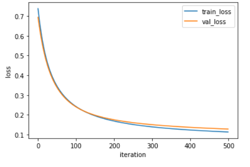
ii) 배치크기 - 128
minibatch_net = MinibatchNetwork(l2=0.01, batch_size=128)
minibatch_net.fit(x_train_scaled, y_train, x_val=x_val_scaled, y_val=y_val, epochs=500)
minibatch_net.score(x_val_scaled, y_val)
# 0.967032967032967

plt.plot(minibatch_net.losses)
plt.plot(minibatch_net.val_losses)
plt.ylabel('loss')
plt.xlabel('iteration')
plt.legend(['train_loss','val_loss'])
plt.show()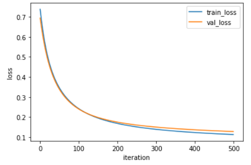
Conclusion.
거의 차이가 없는 듯이 보이지만 배치크기가 128일 때 그래프가 좀 더 완만한 것을 확인할 수 있었다. 즉 128일 때 손실값이 줄어드는 속도가 32일 때 줄어드는 속도보다 느리다.
Reference.
도서 <Do it! 정직하게 코딩하며 배우는 딥러닝 입문> 이지스 퍼블리싱, 박해선 지음
colab에서 google drive에 있는 파일에 접근하는 방법
Google Colaboratory 입문자들을 위한 설명!
추후 BERT로 classification하는 문제를 풀어보고 싶은 분들은 아래 링크에 매뉴얼을 참고하여 실습해 보시기 바랍니다. https://jisoo-coding.tistory.com/34 BERT를 Google Colab에서 돌려보기(TPU 사용) 글에..
jisoo-coding.tistory.com
stackoverflow.com/questions/48905127/importing-py-files-in-google-colab
Importing .py files in Google Colab
Is there any way to upload my code in .py files and import them in colab code cells? The other way I found is to create a local Jupyter notebook then upload it to Colab, is it the only way?
stackoverflow.com
끝.
'Deep Learning > [Books] Do it! 정직하게 코딩하며 배우는 딥러닝 입문' 카테고리의 다른 글
| 다중분류 다층신경망 구현하기 - 하 (1) | 2020.10.29 |
|---|---|
| 다중분류 다층신경망 구현하기 - 상 (0) | 2020.10.19 |
| Python으로 다층신경망 구현하기 (0) | 2020.10.12 |
| [모델 튜닝] K-폴드 교차검증 (1) | 2020.10.04 |
| [모델 튜닝]하는 법 2 - 가중치 제한(feat. L1, L2규제) (0) | 2020.09.28 |